Two weeks ago I presented a global methodology to quantitatively decompose the spectra of mixtures into their respective components providing that their raw spectra were known (aka measured separately). Today I’m presenting some experimental results based on this technique to measure the kinetics of a well-known organic reaction: the esterification reaction.

The reaction itself is relatively basic and involve mixing a carboxylic acid (RCOOH) with an alcohol (R’OH) to produce the corresponding ester (RCOOR’) and water (H₂O).The reaction is presented in Figure 1. Here I used conc. acetic acid (R=CH₃-CH₂) and ethanol (R’=CH₃-CH₂) to produce ethyl acetate.

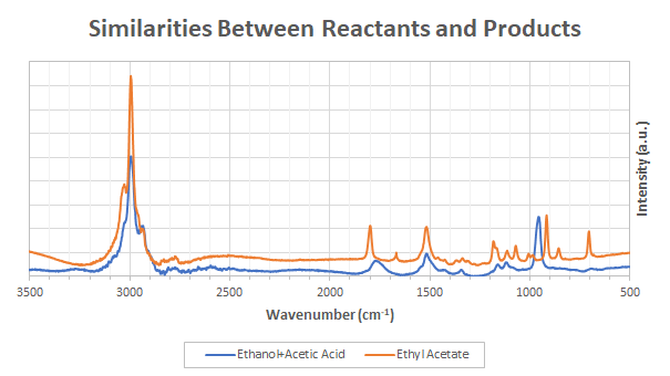
One of the challenges of resolving the various compounds in the esterification process is that the ester (the product) does not differ a lot from the reactants (mixture of acetic acid and ethanol) as most of the chemical bonding are conserved. The few bonding that changes are the -OH in the reactants and the C-O-R’ formed by the ester. In Raman spectroscopy, -OH are almost invisibles and we therefore expect very few changes in terms of number of peaks. On the other hand, the positions of the peaks are expected to shift slightly due to the modified structure of the molecule but this is a second order effect.

Experimentally, the spectra of pure ethyl acetate, ethanol and acetic acid were measured. The difference between the product and reactants spectra are shown in Figure 2. As expected, the two spectra are very similar.

A second challenge with the esterification reaction is that it is extremely slow. Even with the presence of a strong catalytic acid like HCl, the reaction takes more than 1 day to achieve completion at room temperature. Tracking variations of the order of 1% therefore requires the laser to be stable enough over long period of times. Also, diurnal temperature changes in the liquid or cloudification of the sample can greatly affect the resulting Raman signal intensity. Finally, the third challenge is that a part of the product (water) is not measurable through Raman spectroscopy. Measuring kinetics however requires to know the exact composition of the mixture (including water) and some heuristic will therefore be required to estimate the amount of water.

Nonetheless I decided to test the reaction to show the strong potential of the OpenRAMAN spectrometer!

7.920 grams (0.106 mols) of 80% acetic acid were added to 5.145 grams (0.107 mols) of 96% distilled ethanol in a beaker. A few drops of 20~29% HCl were added to the beaker as catalyser. The solution was mixed by repetitive sucking with a pipette and 2 ml transferred to a test vial. The vial was closed using paraffin and placed in the OpenRAMAN spectrometer for 36 hours. The laser was set 297.30 mA (about 20-25 mW) and the TEC driver tuned to 22.50°C. The laser was allowed to warm up for 20 minutes before the experiment was run. 10 sec exposure images with 3 dB gain at 16 bpp depth were recorded every 1 minute during the full experiment duration (36 hours) and analysed in Matlab using the process described in my previous post. The initial amount of water was 0.099 mols and the volume was about 14 ml (not measured precisely).

The spectrum of acetic acid was divided by 0.80 to account for the presence of water and the spectrum of ethanol was divided by 0.96 as well. The heuristic used to estimate the amount of water (since it is not measurable through Raman spectroscopy) was to compute the residual of the amount of acetic acid (AcOH), ethanol (EtOH) and ethyl acetate (EtOAc):

with χ_A the molar fraction of the compound A.

This is not the best heuristic for sure to estimate the amount of water as it is sensitive to both the loss of reactants by evaporation, the cloudification of the liquid, the change in laser intensity and the potential change of Raman activity due to diurnal temperature changes. However, it was the best I could come up with.

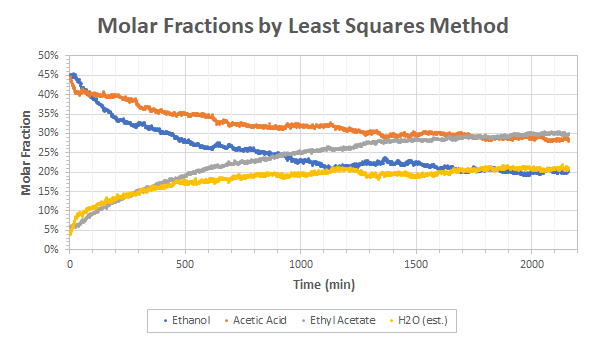
The raw data obtained from the least square method plus the heuristic for the water is given in Figure 3. The trends observed are the expected ones: ethyl acetate and water increase over time while acetic acid and ethanol decreases. All the values reach a non-null steady state that is bound by the equilibrium constant of the reaction.

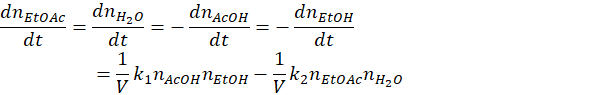
The aim of the conducted experiment is not only to observe the evolution of the various chemicals but also to derive the kinetic constants to further predict the rate of the reaction when reproduced on a larger scale. The form of the kinetic model falls beyond the scope of this post but it is directly related to the slowest step of the reaction of Figure 1 which involve the presence of all the species under the form

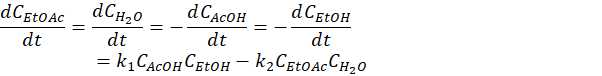
with C_X the concentration of the compound X and k₁/k₂ the rates of the reactions.

Multiplying by the volume, V, twice gives the relation in terms of moles n_X

And further dividing twice by the total number of moles n₀ gives the relation in term of molar fraction

Or (defining new constants)

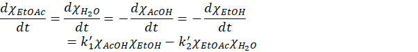
There are therefore two competing reaction taking place: the forward reaction produces ethyl acetate and water at the rate k₁ and depends on the product of the concentration of acetic acid and ethanol and the second reaction decompose the products back into acetic acid and ethanol at the rate k₂.

The model involves two constants but they can be related to another property, K_eq. Indeed, after a sufficiently long time, a steady state will be obtained with a perfect equilibrium between the forward and backward reactions such that

And therefore

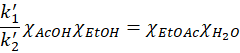
We define K_eq as

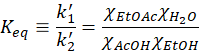
Generally speaking, the right-handed side term is called the partition constant of the reaction. Only at steady-state the partition constant is called the equilibrium constant.

Plotting the partition constant vs. time for the data of Figure 3 gives the results of Figure 4. If we assume that the compounds have reached equilibrium after 2000 minutes, K_eq would be about 1.05 for this reaction.

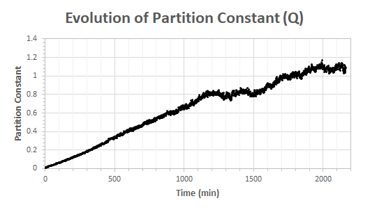
The results of Figure 4 are a bit off from the literature which lists a value of 3.92. It is nonetheless not so bad approximation knowing that chemical reactions have equilibrium on scales larger than 10¹⁰! Two hypotheses can be made to explain this difference:

(1) The reaction may have not achieved pure steady state. This is possible looking at Figure 4 but we are probably not so far from equilibrium when we look at Figure 3.

(2) The molar fractions of Figure 3 are not correct. This is more than likely because we expect that the same number of moles of ethyl acetate and water should be produced and that the same amount of ethanol and acetic acid should be consumed but this is not the case in Figure 3. Both the production and consumption of ethyl acetate and acetic acid seems to be under-estimated compared to water and ethanol contents. I don’t think this could be explained by a discrimination issue between acetic acid and ethyl acetate but rather by the fact that the data returned by the least-squares methods are not molar fractions but a different numeral that is more or less related to but not strictly equal to molar fractions. I still have to investigate on this.

Knowing that there is some discrepancy between the observed fractions and the reality, I performed a fit of the kinetic model on the data of Figure 3 to find the value of k’₁ (since k’₂ can be found from K_eq). I obtained the value 0.0021 min^-1 and 0.0019 min^-1 respectively. With an initial number of moles n₀ of 0.312 mol and a volume of 14 ml, the kinetics constants are found to be k₁=7.8×10^-4 M^-1s^-1 and k₂=7.1×10^-4 M^-1s^-1. I don’t have figures from the literature to compare these values unfortunately.

The fits are shown in Figure 5.

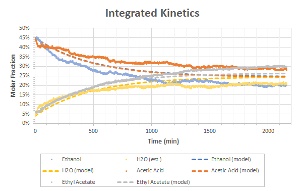
Although the fit is not perfect, the trend is relatively good and the order of magnitude of the reaction rates k₁ and k₂ are certainly correct.

I would have definitively liked to get a 100% match between the fit and the raw data but I will have to find the relationship between the least-squares coefficients of the spectra and the molar fraction first. Still, this is extremely encouraging results as we managed to show that OpenRAMAN is clearly capable of tracking the kinetics of reactions even in challenging conditions such as these ones.

I will come back soon with more investigations on the missing relationships and more experimental data! I would like to give a big thanks to James who has supported this post through Patreon. If you’d like to support me too and get credits as well as many other stuff, consider donating 🙂 You can make the difference!