Robust Calibration Method for Spectrometers
A few months ago I presented the Spectrum Analyzer Suite software with its semi-automated, robust, calibration technology. I’m now taking the occasion of a few days off to detail the algorithm I used there. I haven’t found previous references for such a procedure in the literature, so it’s possible that the method presented here is new.
Generally speaking, the calibration is performed using a calibration lamp. Depending on the spectral range, different lamps can be used. For Raman spectroscopy with a 532 nm, a Ne lamp is a good starting point. It is possible to buy cheap (0.10€/pcs) Ne lamps like I did or buy a professional calibration lamp like Ocean Optics NE-II lamp which costs about 700€ (ex-VAT). Unless you are doing super-precision work, the cheap Ne lamp is good enough.
One of the big challenges of spectral calibration is to deal with missing peaks in an automated way. When working in R&D, one can satisfy to tell which peak is which and then perform a standard polynomial regression, but this method is clearly not suited for day-to-day usage where spectrometers calibration may have to be checked regularly. Ideally, the system should be presented with a spectrum of a calibration lamp and determine itself the proper regression model. This is not necessarily easy to do because the spectrum may lack some of the peaks because they are either too dim or simply clipped by the spectral range of the spectrometer.
The algorithm developed here was found to be extremely robust and is currently semi-automated. It is possible to make it fully automated by using a better peak identification method. In OpenRAMAN, the fit produces a calibration with a typical rms error of 3 pm for a spectrometer resolution of 0.25 nm. No need to say that this is a really good performance.
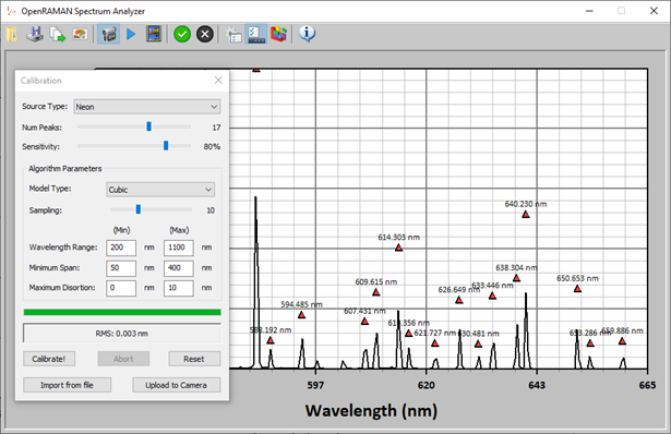
Figure 1 shows a screenshot of the program performing a calibration on a Neon spectrum.

The method itself is divided into two parts: (1) peaks identification, and, (2) model regression. I will only briefly mention peaks identification here and focus on the model regression part.
The peaks identification part of the algorithm will, as its name suggests, find the position of some (or all) of the peaks in the spectra. The user inputs the number ‘n’ of peaks that he would like to find and the system will look for the largest ‘n’ peaks in the spectrum. This value ‘n’ can be lower or equal to the actual number of peaks but should never be larger. Indeed, the regression model part of the algorithm was designed to cope with within peaks very well but is not robust at all to erroneous peaks. So it is better to give fewer peaks to the algorithm and focus only on the major ones.
The peaks identification algorithm will perform the following steps until ‘n’ peaks have been found:
Step 1. Find the maximum intensity ymax in the spectrum that is not masked (see below).
Step 2. Walk to the right of the peak until the spectrum reaches a minimum value ymin.
Step 3. Define a threshold value yth=ymin/κ, with 0<κ≤1, and continue moving to the right until the spectrum goes above the value yth. Mask all the points between the peak and the previous pixel.
Step 4. Repeat the same procedure but this time going left to the peak.
This will identify ‘n’ peaks in the spectrum without being too sensitive to noise thanks to the κ parameter which is typically set to 0.80 by default in the software. It is nonetheless recommended to apply a boxcar smoothing to the spectrum and to perform and background removal first for best results.
Note that the peak positions are rarely used directly as-is because they would limit the performance of the fit. It is recommended to do a sub-pixel estimation of the actual center of the peak by fitting a parabola on the three points around the center. That is, if the maximum was found at position x0, this requires solving the problem

The sub-pixel center position is then given by

Once enough peak positions have been found, we can proceed to the regression of the calibration model.
We start with a set of peak positions <xi>, given in pixel coordinates, that we would like to match to a list of known peaks for the calibration lamp. For the Ne lamp, these known peaks are:
<Ne> = {585.249, 588.189, 594.483, 597.553, 603.000, 607.434, 609.616, 614.306, 616.359, 621.728, 626.649, 630.479, 633.443, 638.299, 640.225, 650.653, 653.288, 659.895, 667.828, 671.704, 692.947, 703.241, 717.394, 724.517, 743.890} (nm)
I would like to recall here that not all of these peaks have to appear in the spectrum for the calibration.
The procedure is to assume a transfer function f(x) that converts from sensor pixel coordinates to spectral coordinates in nanometer and to define a cost-function as

where the function δ(p) is defined as

That is the function δ(p) returns the distance in absolute value between the coordinate p and the closest peak from the set of the Neon peaks list. The cost function is therefore the sum of all the distances between the projected peaks f(xi) and their closest match in the official Neon peaks list. An optimization algorithm will then select the function f(x) that minimizes the cost ε. I will come back on this later.
You can picture the function δ(p) as a series of upside-down triangles connected to each other defining hills and valleys. With the proper function f(x), all the peaks of the recorded spectrum will fall in these valleys. An incorrect function f(x) will have some of the peaks on the hillside and the goal of the optimization function is to drive all the peaks to the valleys.
Isolated peaks, therefore, have a much stronger influence on the fitting because they can potentially generate much larger δ(p). This is a wanted behavior for the algorithm because fitting two isolated peaks is much more meaningful than fitting a close-by doublet.
So far I just talked about f(x) as being a transfer function that converts from a pixel position to a spectral position (in nanometer). A relatively naïve choice would be to use a polynomial of order z

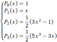
But a better choice would be to use Legendre polynomials

with

These polynomials are orthonormal over the space [-1,+1] which makes optimization function faster to converge and are less likely to produce spurious results. In practice, I tested both approaches and obtained a fit about 10% faster using Legendre polynomials.
In the Spectrum Analyzer Suite, I decided to use linear (z=1) and cubic models (z=3) for the fit. A linear fit will be much faster and gives satisfactory results here because the dispersion of the spectrometer is almost linear in the wavelength range that it covers. On the other hand, a cubic fit will be more general and gives just an extra better calibration with the OpenRAMAN spectrometer. I do not recommend using a higher number of polynomials because it is unlikely that your dispersion will diverge strongly from a cubic model and it will make the system very slow to converge. Also, I recommend to always use an odd order for the polynomials such that you always have a symmetric and an asymmetric basis to fit to your data.
Concerning the cubic model, the basis is

where the coordinates are normalized to the [-1,+1] space.
Since we have ‘N’ pixels in our sensor and that 0≤x<N, we can normalize the coordinate and express the function f(x) as

The coefficients ci are what we will be optimizing.
Before looking at the optimization algorithm, let us interpret the actual meaning of the coefficients ci. Let’s focus on the two first coefficients.
We know that the function f(x) transforms a sensor pixel coordinate into a spectral coordinate (in nm).
The linear model is

That we can re-arrange as

This is also a linear model that has a slope of c1’ and a base offset of c0’ but this time with non-normalized coordinate x. In our application, c1’ is therefore the dispersion of the spectrometer in nm/px and c0’ is the minimum wavelength of the system.
We can re-express the model as

or, put differently,

and therefore

which means that the coefficient c1 in the model is half of the span of the spectrometer and the coefficient c0 the center wavelength. Similarly, the coefficients c2 and c3 will be the maximum departure, in nm, at the edge of the spectrum.
Based on this analysis, we can use the estimation of the span and center wavelength as a starting point for a local optimization method like the simplex (Matlab fminsearch).
Although this does work when the spectrometer is almost perfectly aligned and the design parameters are known, it will not necessarily converge to a global minimum when the spectrometer is not aligned properly or when the design parameters are only loosely known. In such a case, a global optimization method needs to be used. This is the approach taken in the Spectrum Analyzer Suite.
In the software, the user inputs a range of wavelengths (by default from 200 nm to 1100 nm), a range of spans (by default from 50 nm to 400 nm), and a range of distortions (by default from 0 nm to 10 nm). The software will then generate a large number of random starting conditions {c0, c1, c2, c3} that are compatible with the provided range and applies a local optimization to these sets. Any result that is not consistent anymore with the provided range (after optimization) is discarded and the solution giving the best ε is returned. Note that the boundaries given here are super large because I wanted the software to work with almost any dispersion-based spectrometer, not just OpenRAMAN.
Also, it is important to prune solutions after optimization as well because spurious cases like c1=0 will obviously give ε=0 given the proper c0.
The number of systems to generate depends on the dimension used for the model (z+1 so 2 for linear and 4 for cubic). By default, a density of 10z+1 is used in the software.
On my old laptop (5yr+) the algorithms converges to a 3 pm RMS model within 4 seconds for the cubic model and almost instantaneously for the linear model. The algorithm was found to be very robust to missing peaks and still work perfectly with only half of the peaks given.
If you would like to know more about the implementation details, you can download the full source code of the software here.
This is all for today! I hope you enjoyed this post even if it was a little bit more theoretical 🙂
I would like to give a big thanks to James, Daniel, Mikhail and Naif who have supported this post through Patreon. I also take the occasion to invite you to donate through Patreon, even as little as $1. I cannot stress it more, you can really help me to post more content and make more experiments!