Breadboard Version Assembly
This page describes the assembly procedure of the OpenRAMAN breadboard. The breadboard is the development version of the spectrometer and does not focus on cost optimization yet but allows to build a basis that can easily be upgraded to test new concepts. A complete bill of material is given at the end of the page.
The version presented on this page does not meet the strong requirements that we have put on SNR and resolution yet but already allows to produce good spectra of liquid samples.
WARNING: Before we move on I have to warn you that this breadboard uses a laser at the limit of Class 3b. Don’t operate the setup without a good understanding of laser safety. Always wear laser safety goggles designed for the laser being used. Here, I can recommend Thorlabs LG3 laser safety goggles. Don’t fuck up with safety.
The starting point is to print or machine the optical base plate. You can download the STL file of the optical base plate here. I do not recommend FDM printing for the base plate but rather a professional SLS-type print. Once you have your optical base plate, you will have to insert M4x6 helicoils at the marked locations:
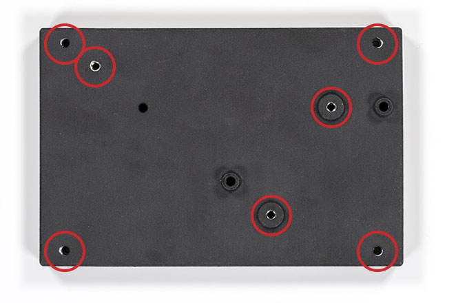
You do not need to add the corner helicoils if you do not plan to fix the optical base plate later. You can also group the order and order the vial holder too (download it here). You will need to hold a lens in the vial holder using a nylon-tip set screw and one more helicoil like this:
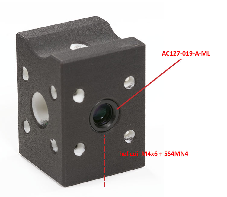
You may have to clean up the holes with the proper end mills depending on the quality of the manufacturing of the SLS part. This is why the holes in my part are smooth and white.
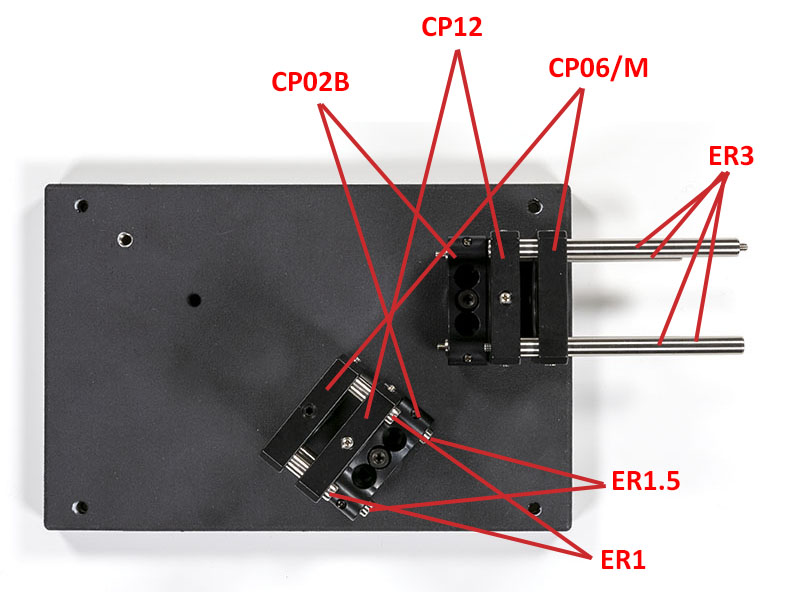
Once this is done you can assemble the optics craddles on the optical base plate:
Next, you will have to assemble the slit assembly with its lens:
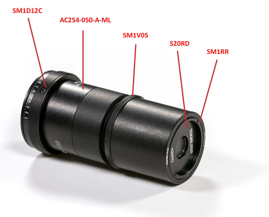
All the parts are standard COTS elements from Thorlabs. The slit can be aligned at infinity using an autocollimator such as described in the tooling page. Don’t forget to close the iris to 12 mm before doing any alignment. Once the slit is aligned, tighten the retainer ring of the SM1V05 part.
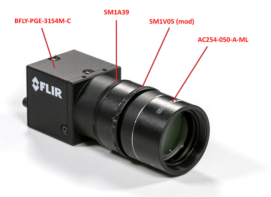
In a similar way, you can now assemble the imaging optics and the camera. The focusing is done with the autocollimator. A small difference here is that the SM1V05 part had to be modified on a late by cutting both ends of the part.
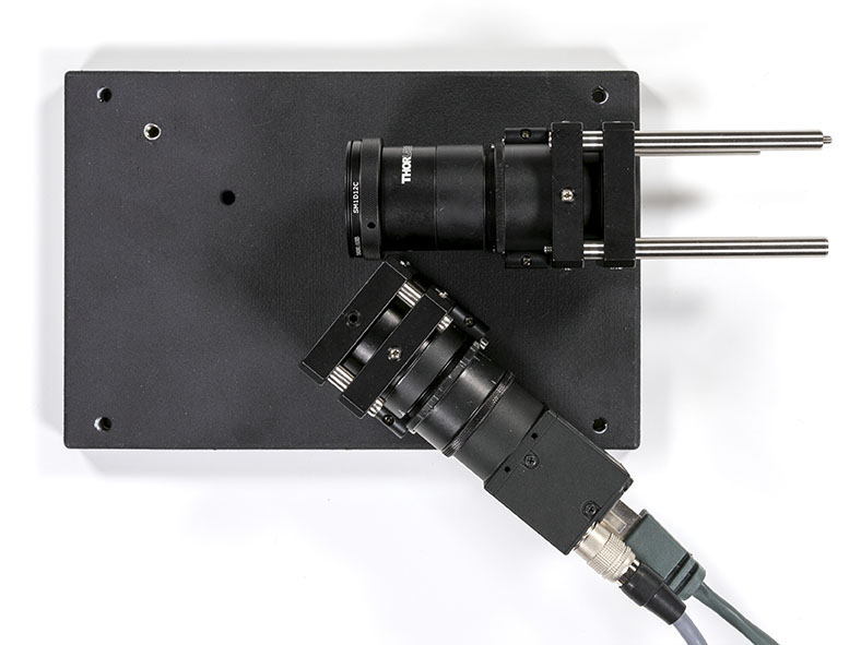
You can now put the slit and camera assemblies in their respective craddles on the optical base plate. The elements should rest on the CP06B for later tuning.
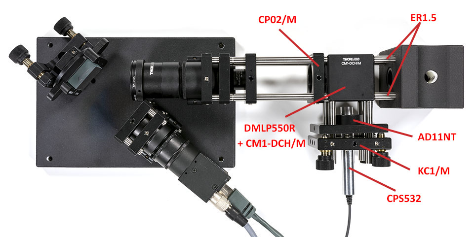
Once the elements have been secured you can plug the camera on and add the grating on the optical base plate:
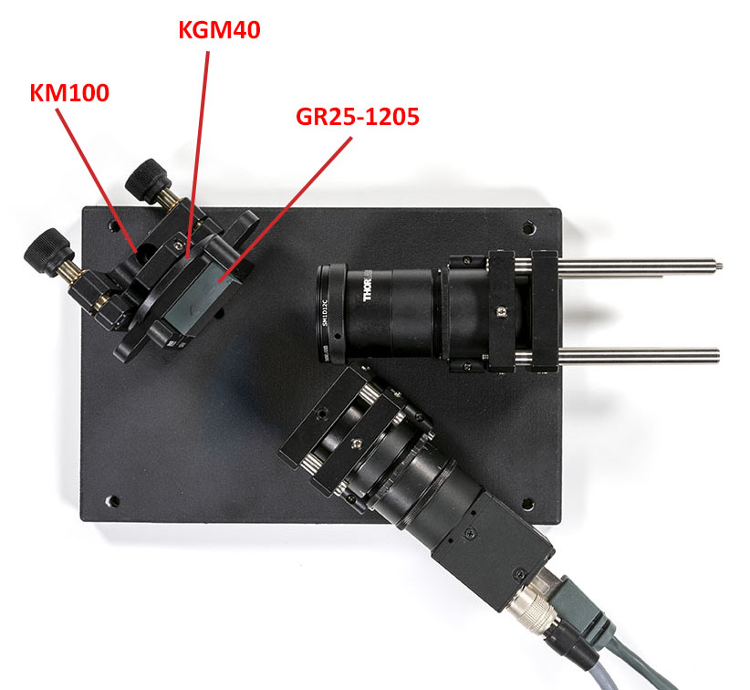
Check the blaze direction when installing the grating. The arrow should point from the slit assembly to the camera assembly.
Once the grating is in place you can add the refocusing lens and align it using the autocollimator. If you do not see the the slit properly a good trick is to remove the grating and put a light with a diffuser behind the iris. You may notice that the lens is in the wrong orientation here but it is not possible to put a mounted lens the other way around easily. I will do an upgraded version for this later.
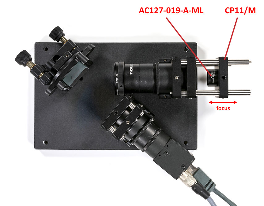
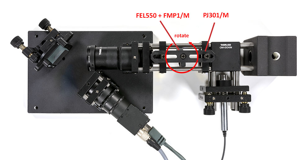
Once the lens is in focus, assemble the rest of the setup. Leave a gap for the edge filter that we will add later on:
We will now align the spectrometer using a neon light bulb placed in the vial holder. You may want to wrap your entire setup in black anodized aluminum foild because the neon light is not really strong (it is however still much brighter than your Raman signal!).
To align the spectrometer, follow these steps in this precise order:
- Turn on the Neon source and shut down all lights. The room should be completely dark. Open FlyCapture program and set the “mirror mode” in settings. Set the camera to Mono 16 bpp. Put the exposure time to 100 ms and set the gain at maximum.
- Untighten the grating screw and turn the grating manually until you see the zero order. Hint: the grating should almost face the slit assembly at that moment. Slowly turn the grating until you see the first line appearing and center them horizontaly in the image. Tighten the screw again. Adapt the gain until the lines are not saturating anymore.
- Unlock the camera assembly screw and rotate the camera until all the lines disperse horizontaly. It is not important if the lines themselves are tilted. Relock the camera assembly screw once the dispersion is horizontal.
- Unlock the slit assembly screw and rotate the slit assembly until the slit are perfectly verticals. You can use the camera monitor program crosshair overlay to help you. Once the lines are perfectly vertical you can lock the slit assembly again.
- Using the grating kinematic mount knobs, center the lines vertically and bring the first spectral line at the position X=779 px. The cursor position is displayed at the bottom of the camera monitor program.
- In FlyCapture, set the ROI to 200 px height and center the ROI. Then save the user settings to the first channel such that the camera will keep these settings for the next time you power it up.
Your spectrum should now look like this:

Now put the edge filter in place and put a white light in place of the sample with a diffuser in front of it. Turn the edge filter until the first few pixels on the camera becomes black. This allows to tune the cut-on wavelength to reach ~540 nm instead of the nominal 550 nm of the filter. Alternatively, you can substitute the white light by a fluocompact lamp since it has two intense peaks at 542 and 546 nm. Rotate the edge filter until the first line disappear but the second line is still visible.
Once the spectrometer is properly aligned and the edge filter tuned correctly, we will stir the laser to form a spot on the slit. If you omit this step, the tiny laser spot will likely end up out of the clear aperture of the slit and you will not measure anything.
Stirring the laser can be somewhat complicated but a very convenient way to proceed is to use Rhodamine B dye. Be very careful however when using Rhodamine B powder because it will dye in pink anything it comes in contact to! Wear gloves, respiration mask and eye protections. Avoid producing mist in the air and wash everything after usage. Also, you will need only a tiny amount of Rhodamine B, only a few milligrams will be sufficient. Your sample should look like that:
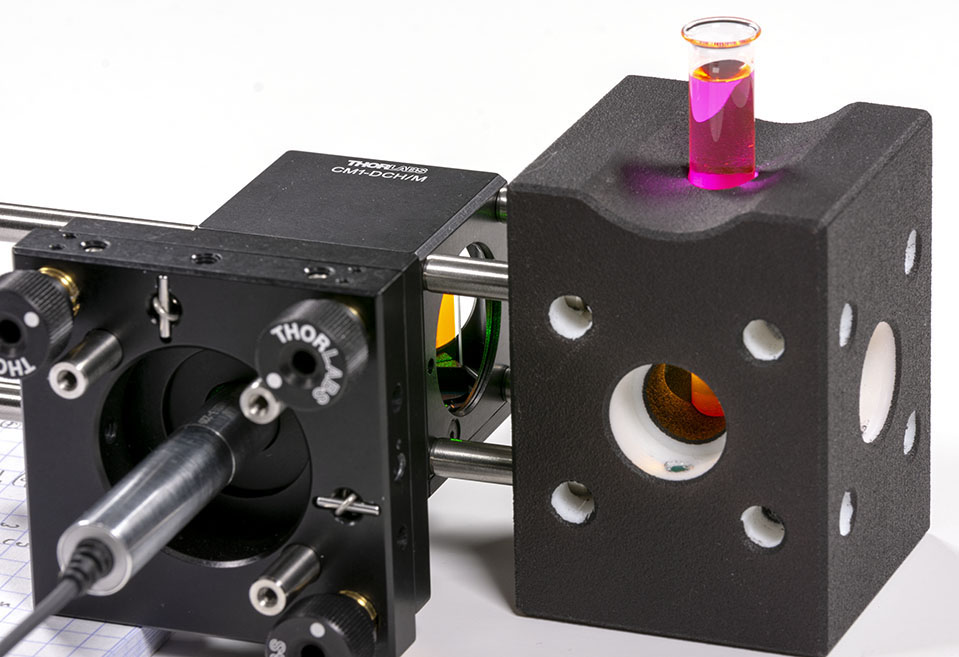
One of the very nice thing with Rhodamine B is that it has very strong fluorescence in the exact wavelength range that we are looking at when exposed with our DPSS laser. This allows to use small integration time on the camera and catch the signal in realtime easily. Rhodamine B also allows to see the path of the laser light in the vial:
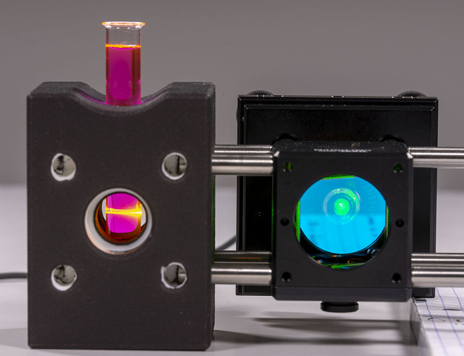
Be carefull if you want to look at the setup when the laser is on and always wear your laser safety googles.
To stir the laser I recommend moving the beam horizontaly until you catch the signal on your camera monitor program. Then stir the laser vertically to be at the center of the slit by estimating the upper and lower boundaries of the slit.
If you are a perfectionist, you can tune the camera assembly orientation and the grating tilt using the signal from the Rhodamine. If you choose to do that, you will have to put back the neon lamp to realign the slit and then retune the grating such that the first spectral line ends up at its correct position. I personnaly recommend doing these fine tunes.
Once you are confident you Raman spectrometer is completely aligned, you can measure real samples with it! To measure a sample, follow this procedure:
- Put your liquid sample in a clean vial. The sample should be clear without any bubbles.
- Go in the camera monitor program and set exposure time to its maximum value (1 second here) and adapt the gain such that your image does not saturate.
- Record images for 1 minute (or longer) in the camera monitor program.
- Wash the vial with water several times and measures the signal with water in the exact same conditions (exposure time, gain, number of images…)
- Run the Matlab script to extract the Raman signal. You may have to tune the wavelength range in the program depending on your own alignment.
- Eventually remove the background line using a third-party program. I got satisfactory results using the Matlab script BACKCOR written by Vincent Mazet. You can find his script on the Mathworks website.
Here is an example of a 1 minute exposure spectrum of acetone compared to a professionnal spectrum obtained at the SDBS database:
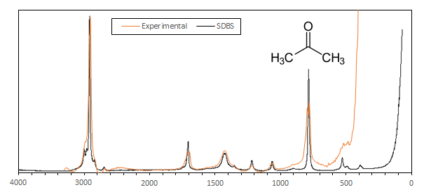
The resolution is about 34 cmw-1 and the SNR is pretty good. This particular spectrum was obtained on a spectrometer where the edge filter was not aligned at its best which explains the loss of resolution below 600 cm-1
A Bill of Material for the breadboard version can be found here-below:
The total price is € 2,464.46 ex-VAT at the moment, excluding non-recurring costs and consumables such as tooling and vials. Cost reduction will be addressed during the prototyping phase.
The vials can be bought from FIERS chemicals and costs about 2 cents each (ref HC01.1). It is not mandatory to change the vial each time if you are not doing analytical research.
To retrieve the spectrum from the recorded images, you can use this Matlab code:
%% main program
%% copyright OpenRAMAN (C) 2018, All Rights Reserved

% init
clear all, close all, clc

spectrum = load_spectrum('EtOH')' - load_spectrum('water')';

% filter
%window_size_highpass = 1000;
window_size_lowpass = 3;
polyfit_order = 3;

if exist('window_size_highpass') && window_size_highpass > 0
    spectrum = spectrum - filter(ones(1, window_size_highpass) / window_size_highpass, 1, spectrum);
end

if exist('window_size_lowpass') && window_size_lowpass > 0
    spectrum = filter(ones(1, window_size_lowpass) / window_size_lowpass, 1, spectrum);
end

if exist('polyfit_order') && polyfit_order > 0
    spectrum = spectrum - polyval(polyfit(1:length(spectrum), spectrum', polyfit_order), 1:length(spectrum))';
end

% set zero
spectrum = spectrum - min(spectrum);

% get size
num_points = length(spectrum);

% build wavelength axis
x = 1:num_points;

wavelengths_axis = 540 + 0.057479061 * x;
cm1_axis = 1e7 .* (1 / 532 - 1 ./ wavelengths_axis);

figure(1)
plot(cm1_axis, spectrum)
axis([0; 4000; 0; Inf])
set(gca, 'XDir', 'reverse')
drawnow

%% function to load spectrum from tif files
%% copyright OpenRAMAN (C) 2018, All Rights Reserved
function avg_bin_filtered = load_spectrum(exp_folder)

    % consts
    bin_width = 1;

    % get info on images
    ls = dir(fullfile(exp_folder, '*.tif'));

    num_images = length(ls);
    im = imread(fullfile(exp_folder, ls(1).name));

    [height, width, ~] = size(im);

    % mean and std
    im_sum = zeros(height, width);
    im_sum_sq = zeros(height, width);

    for i=1:num_images
        im_curr = double(imread(fullfile(exp_folder, ls(i).name)));

        %im_curr = medfilt2(im_curr);

        im_sum = im_sum + im_curr;
        im_sum_sq = im_sum_sq + im_curr.^2;
    end

    im_mean = im_sum / num_images;
    im_std = sqrt((im_sum_sq / num_images) - im_mean.^2);

    % recompute mean by removing 5% outliers
    k = 1.96;

    im_sum = zeros(height, width);
    im_count = zeros(height, width);

    for i=1:num_images
        im_curr = double(imread(fullfile(exp_folder, ls(i).name)));

        %im_curr = medfilt2(im_curr);

        mask = zeros(height, width);
        mask(abs(im_curr-im_mean)<=k*im_std) = 1;

        im_sum(mask>0.5) = im_sum(mask>0.5) + im_curr(mask>0.5);
        im_count = im_count + mask;
    end

    im_sum = im_sum ./ im_count;

    % binning
    avg_bin = zeros(1, floor(width / bin_width));

    for x=1:width

        id = 1 + floor((x - 1) / bin_width);

        avg_bin(id) = avg_bin(id) + sum(im_sum(:,x));
    end

    % save result
    avg_bin_filtered = avg_bin;

end